GIF Animation (138KB)
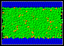
Fig. 1 A snapshot of liquid argon between parallel solid surfaces.
The potential between argon molecules was represented by the well-known Lennard-Jones (12-6) function as
The solid surface was represented by 3 layers of harmonic molecules (1020 molecules in each layer) in fcc (111) surface. We have controlled the temperature of the solid surface by arranging a layer of phantom molecules outside of 3 layers. This technique mimicked the constant temperature heat bath which conducted heat from and to the 3rd layer as if a bulk solid was connected.
The potential between argon and solid molecule was also represented by the Lennard-Jones potential function. In our previous study on the liquid droplet on the surface, we have found that the depth of the integrated effective surface potential eSURF was directly related to the wettability of the surface. Hence, we used a quite wettable potential parameter (eINT = 0.894x10⁻²¹ J) on the top surface to prevent from bubble nucleation and changed the wettability on the bottom surface as in Table 1. The solid surface became more wettable from P2 to P5.
| Label | eINT (x10-21J) | e*SURF | qDNS (deg) | qPOT (deg) | |
|---|---|---|---|---|---|
| P2 | 0.467 | 1.65 | 118.7 | 117.1 | |
| P3 | 0.610 | 2.15 | 82.7 | 78.1 | |
| P4 | 0.752 | 2.65 | 60.2 | 53.4 | |
| P5 | 0.894 | 3.15 | - | - |
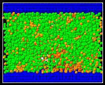
As an initial condition, an argon fcc crystal was placed at the center of the calculation domain. After the system was run for 500 ps until the equilibrium argon liquid was achieved, we gradually expanded the system volume by moving the top surface at a constant speed. We could observe the bubble formation and growth.
In order to visualize the density variations leading to the vapor bubble nucleation, we have applied three-dimensional grids of 2Å intervals and visualized the grid as a 'void' when there were no molecules within 1.2sAR. An example of such a void view representation is shown in Fig. 2(b) in comparison with the sliced view (Fig. 2(a)). Obviously, the assemble of such voids effectively represents the real void in the liquid.
 | 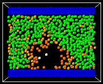 |  |
| (a) Full View | (b) Sliced View | (c) Void View |
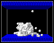
Animations of void patterns for each conditions are shown in Fig. 3.
 149KB |  142KB |  133KB |  136KB |
| P2 | P3 | P4 | P5 |
Small void appeared and disappeared randomly in space and time but preferentially near the bottom surface. Finally, one of the void successfully grew to a stable vapor bubble on the bottom solid surface. It seems that when the void size is as large as 100 voids (related to about the radius of 10 Å), a single stable vapor bubble stayed on the surface.
The size of the largest void in each snapshot is drawn in Fig. 4 as "Bubble Size" in comparison with the pressure variations.
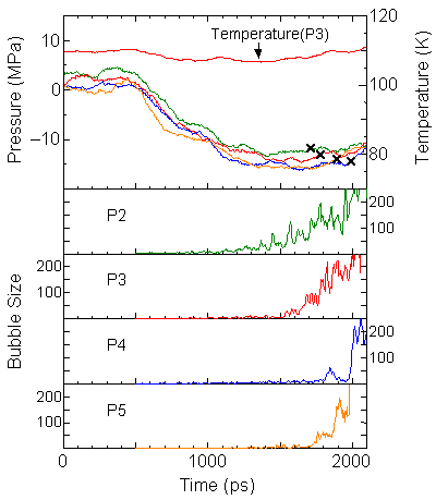
When the bottom surface is less wettable, the size of void seems to increase monotonically, however, each void appeared and disappeared randomly in space. On the other hand, when the bottom surface is more wettable, no large void appeared until the sudden appearance of the void of about more that 100. We defined the nucleation point when the size of void exceeds 100 (cross symbols).
We compared the nucleation pressure for various conditions in temperature-pressure diagram in Fig. 5.
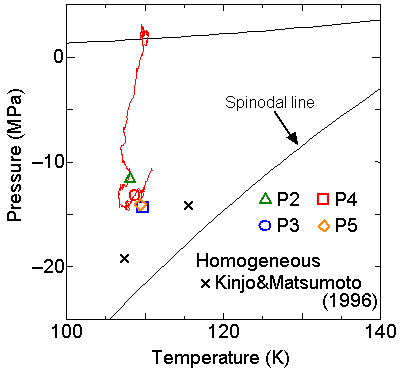
With the increase in the surface wettability, the nucleation pressure approached to the spinodal line (the thermodynamic limit of the existence of superheated liquid, calculated from the equationof state for Lennard-Jones fluid). The result of the homogeneous nucleation simulation is also plotted in the figure. When a very high wettability of the surface was employed, the situation was closer to the homogeneous nucleation as for P4 and P5. With the decrease in the wettability, the nucleation point moved farther from the spinodal line.
After detecting the stable vapor bubble formed on the surface, we repeated the simulation for 400 ps without the volume expansion in order to observe the equilibrium structure of the vapor bubble. Two-dimensional density distributions (Fig. 6) and potential distributions (Fig. 7) are obtained by cylindrical averaging through the center of the bubble.
| h [Å] | 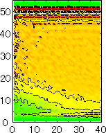 | 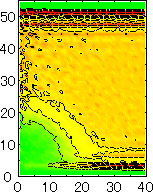 | 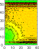 | 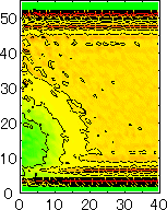 |  |
| r [Å] | r [Å] | r [Å] | r [Å] | ||
| P2 | P3 | P4 | P5 |
| h [Å] | 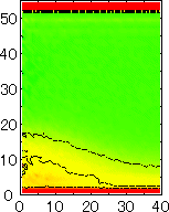 | 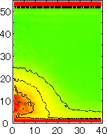 | 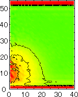 | 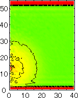 |  |
| r [Å] | r [Å] | r [Å] | r [Å] | ||
| P2 | P3 | P4 | P5 |
The layered structure of liquid near the surface is clearly observed in Fig. 6. On the other hand, except for about two layers near the surface the shape of bubble can be considered to be a part of a sphere. It is observed that the less wettable surface leads to more flattered shape.
We have measured the apparent contact angle by the least square fit of a circle to the density contour line of half of liquid density. Since we have discovered that the cosq was a linear function of the depth of integrated effective surface potential e*SURF for the liquid droplet on the surface, we have compared the present result with the same fashion in Fig. 8. It is obvious that the contact angle was in good agreement with the case of liquid droplet marked as cross symbols.
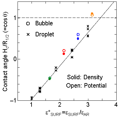
It is interesting to consider the most wettable surface in Fig. 6 P5, in which clearly observed that the layered liquid structure completely covered the surface. As we monitored the position of center of bubble, it stayed at almost the same height from the bottom surface, though the eINT parameter on both surfaces were the same for this condition P5. It is confirmed that the bubble was trapped by the bottom surface. Furthermore, if we extend the definition of the contact angle cosq to Hc / R1/2, the measured point is almost on the line in Fig. 8. Here, R1/2 is the radius of the fitting circle to the half-density contour, and Hc is the center of the fitting circle. This suggests the possibility of characterizing the liquid-solid contact belond the apparent contact angle.